Granger causality analysis -- building a foundation

Previously, I had used a "high level" Granger causality toolbox for the inference of directed edges. While there were some early results, I don't like to leave things as a "black box" without understanding the mechanics. In particular, I had observed that the $p$-values for the Granger toolbox seemed to be incorrectly scaled (which causes the FDR method to break down) and I had some serious concerns about the ability of the MVAR model to capture neural processes. So, I decided to implement Granger causality analysis from first principles, which is VAR modeling of time series data.

Getting started with VAR modeling, I found the Mathwork's tutorial to be really helpful.

Scooped!

My term project has been scooped!

• http://www.ncbi.nlm.nih.gov/pmc/articles/PMC3704386/
• http://www.ploscompbiol.org/article/info%3Adoi%2F10.1371%2Fjournal.pcbi.1002653
• http://www.mit.edu/people/sturaga/papers/TuragaNIPS2013.pdf

Actually, there is quite a bit of work -- especially on PLoS ONE, it seems -- on applying causal measures on neural data (e.g. electrode arrays, etc.).

Lot of recent work also seems to pay a lot of attention to transfer entropy, which I also find very interesting. However, I am leaving the TE as beyond the scope of the CS224w work. I find conceptual similarities between TE and Granger causality.

Project milestone

Still a lot of pieces missing: Project milestone

Undirected edge inference -- temporal filtering

For reference, here is the impulse response of calcium indicators today, taken from the article on GCaMP6:

Time constants are rather high, almost 1 s for the GCaMP6 variants.

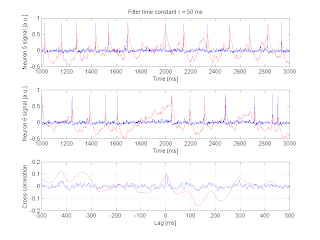
I implemented a basic filtering system, where the impulse response is a simple exponential function characterized with a time constant $\tau$. Here are some representative traces and the filtered output, as well as how the filtering operation modifies the cross-correlation. (The neuron pair shown below are synaptically connected):

It can already be surmised that the temporal filtering will degrade our ability to detect significant correlations. Some thoughts that arise:

• First, it may be the case that the filtering result will depend on the width of the action potential. While the Izhikevich model with the current parameter set produces spikes with reasonable widths, it still may be the case that the widths are dependent on the numerical integration step size.
• Secondly, I wonder if there is a simple closed form formula for determining the resulting cross-correlation when the time series has been temporally filtered. (This seems very plausible.) On the other hand, I'm learning about the limits of cross-correlation for the current task... closed-form formulas for other measures will be harder to obtain.
• Yes, there should be a simple formula here -- will verify soon.
• Thirdly, it appears that we have to "retrain" a $p$-score classifier following temporal filtering.

I now suspect that the "inferrability" of the undirected network will be sharply degraded by the temporal filter. It suggests one line of investigation: is there a mechanism that may allow us to recover the network (e.g. multiple trials, etc.) despite the temporally degraded signals?

I resynthesized the CDF of cross correlations given temporal filtering of $\tau = 5$ ms. It can be seen that the distribution is different from that without the temporal filtering:

Undirected edge inference -- some failure modes

I considered the undirected edge inference task for higher edge densities. My "standard" model currently uses $M=100$, $N=100$, which is a very sparsely connected ($1\%$) network. I considered how the difficulty of the task varies for $M=500$, $M=1000$.

At $M=500$, the inference run finds many more edges than the true number. I think that the cross-correlation does not have the means to distinguish between direct and complex descendant relationships, and that it will tend to close triads. It seems to me that Granger causality would better handle dense graphs (since G-causality asks whether $X_1$ influences $X_2$ when other $\left\{X_i\right\}$ are given).

At $M=1000$, the Izhikevich model itself "locks up," and all spikes become "phase-locked." It appears that the coupling coefficient $\alpha$ that I am using is too high to support such a dense network.

These observations suggest that I should consider a case with lower $\alpha$, as to explore varying edge densities in the inference.

It also suggests to me to try out bipartite populations of neurons with dominant synaptic connections between the parts. This actually models the kind of experiments that I want to eventually undertake.

FDR-based undirected edge inference validation

Right now, I suspect that the G-causality based inference is "too eager" to predict an edge for a given FDR level $q$, while the undirected inference results seems to be better calibrated to $q$. Here, I'd like to explicitly quantify the FDR calibration for undirected edge inference.

Here is a single instance of $N=100$ undirected inference, where I shmoo the FDR level q, and measure the actual FDR observed by the inference method. I also plot the standard ROC of the inference:

Note that the FDR is not the same quantity as the FPR. See the Wikipedia page on ROC for details.

Here is the above graph, based on 50 inference runs:

It is interesting that the undirected inference for the choice of parameters that I've picked for the Izhikevich numerical model performs so well. This way, we can see the effects of temporal filtering on the inference performance!

G-causality analysis of neuron traces

A bit more background on G-causality: Scholarpedia (run by Izhikevich!) article on Granger causality.

I am concerned about the assumption that G-causality analysis makes that the time series can be described as a linear (multivariate autoregressive) model. My initial exploration of the G-causality toolbox is that, while the analysis seems to recover directed edges in the neural network for my initial (small) toy models, that the assumption of the linear model may be invalid for my application. In particular, the toolbox complains that my residuals after the model fit is not white (by the Durbin-Watson test), which suggests that the model is not good for the neural traces.

That said, it does seem to "work". Here, the analysis correctly reproduced three directed edges in a set of five neurons:

Actually, the Durbin-Watson test is not implemented in the toolbox. It always throws a warning... Nevertheless, I still want a sanity check of the validity of the MVAR fit on the neural traces... When I "turn on" the true DW test for residual whiteness, the neural data supposedly passes.

But clearly, the problem here is that I'm just using the toolbox superficially without knowing about its workings... Now, to dig in.

First question to consider is how well the multivariate autoregressive (MVAR) model assumed by G-causality describes the data. As it turns out, the description is quite good, as long as one is careful about the sampling rate of the signal:

(I worry about overfitting here...)

Next, we want to know the maximum lag (the "model order") we should use in the G-causality analysis. Based on the delay in the cross correlations, we should use up to 10 ms of lag:

Making inferences of directed edges with the G-causality toolbox:

Some more inference instances:

It is quite interesting that the Granger analysis can infer directed edges! (Q: So far, I have been using exclusively excitatory synapses. Can the method also pick up inhibitory synapses?)

I find that the "FDR level" knob seems to understate the rate of false positives for the G-causality inference. I am not sure how the toolbox calculated $p$-values associated with each Granger edge, which might be the cause for this discrepancy.

FDR-based inference on Izhikevich simulation using cross-correlation as metric

Simulation of Izhikevich neurons (10 and 100 neurons):

In the above simulation, all neurons are independent (no synaptic connections). Here is a distribution of $C_{ij}^\mathrm{max}$ for uncorrelated neurons (i.e. the "distribution of the test statistic under the null hypothesis"):

Now here is a set of neurons with some synaptic connections between them. (Not easy at all to discern the underlying graphical structure.)

We consider the distribution of $p$-values for synaptic pairs in the Izhikevich model as a function of the "synaptic strength" constant $\alpha$:

The above shows that a synaptic strength of $\alpha \approx 10$ is necessary to discern the connectivity structure in the Izhikevich model. Note that $\alpha \approx 10$ does not yield a totally trivial (i.e. deterministic firing) relationship between two synaptically connected neurons. Here is a trace of two neurons with connectivity of $\alpha = 10$ that shows that the relationship is not necessarily deterministic:

For that matter, $\alpha = 20$ doesn't yield deterministic relations either, but there are more (almost) coincident spikes between the two:

(Note: An independent characterization for the "interpretation" of $\alpha$ could be an empirically derived probability that the post-synaptic neuron fires within some interval of receiving the pre-synaptic spike.)

Next, let's try some inference on a model of $N=10$ neurons with $M=10$ synapses. (My eventual target is to run simulations on $N=100$ or even $N=10^3$ neurons.) I visualize the inference result as an adjacency matrix, where a filled green rectangle represents a correctly inferred edge, unfilled green rectangle represents an uninferred edge (false negative) and a filled red rectangle represents a falsely inferred edge (false positive). All inference instances are for $\alpha=10$.

Also, examples of inference on $N=100$:

Next, I want to obtain the ROC curve.

Granger causality ("G-causality")

Basic intuition: "one series can be causal to the other if we can better predict the second time series by incorporating knowledge of the first one."

Trying out a Matlab package for Granger causality on simulated neural traces. I simulated three traces where neuron 1 drives neuron 2, and neuron 3 is isolated. The G-causality inference produced the correct result:

On the other hand, I don't know how well the traces can be modeled by the multivariate autoregressive (AR) model assumed by G-causality. (The toolbox gives a warning that the residuals after the AR model fit is not white.)